The number of companies startups working in the real-time big data space is pretty stunning (including ourselves). But if you look closely, you see that there are quite a few number of ways to approach that problem. In this post, I’ll go through the different technologies to try to draw a real-time big data landscape.
Unfortunately, real-time has come to mean a lot of things, mostly that “it’s fast”. For this post, let’s focus on event data. It’s probably possible to talk about real-time for more or less static data (like crawled web pages), where “real-time” would then mean that it’s fast enough for interactive queries. In that sense, Google search is probably the biggest real-time big data installation.
So back to event data. To have a common ground, let’s consider this setting: You have some form of timestamped event data (user interactions, log data, sensor data), and you’re interested in counting activities over different time intervals. For example, you’re interested in the most retweeted picture over the last 24 hours, or the average temperature in your cluster for the last hour. Let’s also add the possibility of filtering these counts (only users from Germany, only clusters in that rack, etc.) Much more complex applications are thinkable, of course, but already this tasks allows us to see differences between the different approaches.
In the following, we start with a relational (single server) database as the baseline and then discuss different techniques used to make the system faster. Note that real-world systems often employ a mixture of techniques.
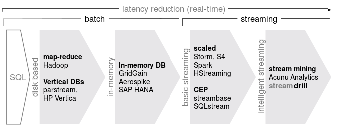
I admit that this image simplifies a lot, it is neither chronologicall accurate, nor does accurately reflect the relationships, but I think it serves as a good big picture to roughly order the different approaches in terms of deviation from the baseline which we’ll handle next:
The Classical Approach: Relational Databases
As a starting point, let’s take a classical relational database. You would
continually insert new events and use queries like SELECT count(*) FROM
events WHERE timestamp >= '2013-06-01 00:00' AND timestampe < '2013-06-02
00:00'.
This is a perfect approach and works well until you have a few million entries in your database. The main problem here are that the database gets slower and slower as you add more data, and that the queries always run a full scan over a significant part of your data set. At some point, these two effects start to amplify one another: Your queries will be slow because there is so much data and inserts become slow because queries are constantly running.
Finally, operations are slow since they are eventually disk based. Even if you factor in caching and RAIDed disks, you won’t be able to go beyond a few hundred inserts per second.
Clustering, Map-Reduce and friends
So if a single server is too slow, let’s make it faster by parallelizing. Luckily, many operations can be parallelized, often even with linear gain in the number of nodes. MapReduce falls into this category, as most NoSQL approaches (although they don’t always come with the query capabilities).
While this approach can lead to impressive performance, there are also a number of things to be considered: Going from a single server to a cluster of servers has some initial performance hit due to network latency, data transfer costs, etc., such that there exists something like a minimum viable cluster size below which the system is not faster than a single server. It might be quite expensive to scale to real-time. Also, as data is constantly growing, one has to keep adding servers to keep the performance on a stable level. The computation is still batch in nature, which means that queries need some time to compute and are therefore not based on the most recent data. There is significant latency in the results.
Hadoop is the most prominent example in this category.
Vertical Databases
One problem with classical databases is that the data is usually stored by rows. So if you want to aggregate over one of the columns (for example, for counting events conditioned on the value in a column), you have to either load a lot of extra data, or you have to do a lot of seeking to only read the required columns.
Vertical databases store the data by columns, so that one can quickly scan all the values of a column. It’s a bit as if one only keeps secondary indices and discards the actual data. One could also store each column in sorted order (keeping pointers so that one can reconstruct the rows if needed), which make range queries even more efficient.
This is an interesting approach, mainly geared at improving disk performance.
Parstream, Shark, Cloudera Impala, HP’s Vertica, and Teradata Aster are examples in this category.
In-Memory
If disk access is the main problem, why not move everything to memory? Together with clustering, and the availability of machines with hundreds of GB of main memory, one can achieve impressive performance improvements (1000 times and more) over disk based systems. Such approaches can also be combined with clustering or vertical storage schemes.
The downside is, of course, that RAM is quite expensive still.
Examples are GridGain, SAP’s HANA.
Streaming
The approaches we have discussed so far are all essentially batch in nature. This gives great flexibility in the queries, but computing results requires a lot of resources. Another approach is to process the event stream as it comes in, aggregating relevant statistics in a way which can later be queried. Results will always be based on the most recent data. This can naturally be combined with clustering to scale the performance.
One issue here is how to make the results of the computation queryable. This usually means that you need some (scalable) storage on the side where you put the results, which adds to the complexity of the installation.
Examples are Twitter’s Storm, Spark, or HStreaming or MapR, which both build this kind of streaming technology on top of Hadoop.
Complex Event Processing (CEP)
CEP is not a performance technique per se but rather a SQL-like query language for streams, which makes it easier for you to work with these systems, as the actor based concurrency model which you find in Storm or others takes a bit of getting used to. Such systems are usually in-memory, and don’t necessarily provide clustering.
I’m also listing this here because CEP systems predate the current Big Data hype.
On the other hand, CEP systems have problems aggregating information over very large spaces. They work best for aggregating a number of key statistics (up to a few hundred) from massive event streams.
Examples include SQLStream, or Streambase, which was aquired by Tibco announced just yesterday.
Approximate Algorithms
So far, all the techniques focus on improving performance through parallelization, using faster storage, or precomputing queries in a streaming fashion. But all these methods don’t touch the original counting task.
Approximate algorithms change that by not giving exact results but trading accuracy for resource usage. I’ve already blogged a lot about stream mining algorithms which do exactly that. Count-min sketches, for example, compute approximate counts using hashing techniques and are able to approximate counts for millions of objects using only very little memory. Moreover, as you supply more memory, results become more exact. These systems are usually in-memory, and also don’t necessarily provide clustering.
The downside here is, of course, that results are no longer exact, which might be either be perfectly ok (e.g. trending topcis) or a dealbreaker (e.g. billing).
Approximate Algorithms are also not strictly restricted to stream processing approaches, you can also use them in a batch fashion to run on data. For example, Klout has a collection of user defined functions to use with Hadoop.
Examples here are our own streamdrill, and Acunu Analytics.
What it says on the box vs. what’s inside the box
Real-time Big Data is an important topic which generates quite a lot of buzz right now. But on closer inspection, there are many different approaches which all have different characteristics when it comes to cost, scalability, latency, and exactness. I think these differences are important when it comes to deciding which solution is the best fit for your specific application, so it’s good to be aware of the differences.
Posted by Mikio L. Braun, Matthias L. Jugel at 2013-06-11 16:45:00 +0000
blog comments powered by Disqus