
What is streamdrill's trick?
In the previous posts I talked about what streamdrill is good for and how it compares to other Big Data approaches to real-time event processing. Streamdrill solves the top-k problem which consists in aggregating activities in an event stream over different timescales and identifying the most active types of events in real-time.
So, how does streamdrill manage to deal with such large data volumes on a single node?
Streamdrills efficiency is based on two algorithmic choices:
- It uses exponential decay for aggregation.
- It bounds its resource usage by selectively discarding inactive entries.
Let's take these two things one at a time.
Exponential Decay vs. Exact Time Window
Usually, when you do trending, you aggregate over some fixed time window. The easiest way to do this is to keep counting and reset the counters at a fixed point in time. For example, you could compile daily stats by taking the values at midnight and resetting the counters.
The problem with that approach is that you have to wait for the current interval to end before you have some numbers, which is hardly real-time. You could take the current value of the counter nevertheless and then try to extrapolate in some way, which is also hard if the rate at which events come in varies a lot.
Another approach is to do a "rolling window", for example, having the counts between now and the the same time yesterday. The problem with that approach is that you need to keep all the data somewhere so that you can subtract an event when it falls out of the window. If you want to aggregate over longer time intervals, say a month, this gets hard, as you have to potentially store millions of events somewhere.
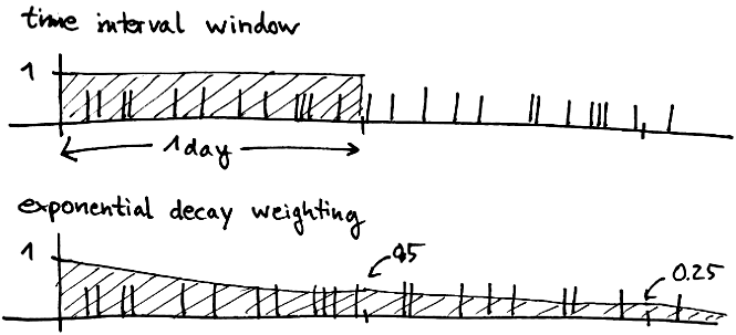
Another approach is to use some form of decay. The idea here is that the "value" of an event decays continually over time until it is eventually zero. That way, you again get an aggregate over some amount of time, although it's not exactly the same thing as a fixed time window. In the end, it doesn't really matter if you understand what it is exactly you're measuring.
The good thing is that decaying counters can often be implemented in a way which does not require us to keep all of the information, but only a few numbers per entry.
Streamdrill does exactly this, using exponential decay. This means that after a specified amount of time, the value of an event has continually reduced to one half, and then again to a quarter, and so on. We chose exponential decay because it has the nice property that a counter always decays to half its original value after a given amount of time, irrespective of the initial value of the counter. That is not the case, for example, for linear decay, where a counter starting at 1000 would take twice as long as one starting at 500.
Keeping resource usage bounded
As I said above, streamdrill throws data away. More specifically, it removes the most inactive entries to make room for new ones. The main purpose of this technique is to ensure that the resource usages of streamdrill are bounded which is important to keep streamdrill's performance constant.
This is also something we've found people having a hard time to digest. After all, isn't the whole purpose of Big Data to never throw away data?
First of all, note that there really is no way around throwing data away if you want to have a system which runs in a stable manner. Otherwise, data will just accumulate and your system is bound to become slower, unless you are able to grow it. But that costs money and adds a layer of complexity to your system you should not underestimate.
Throwing data for inactive entries away also has the nice effect that you focus on the data which is much more likely to make the top-k entries.
Second of all, as I've also discussed in another post, for many applications, in particular if you're really interested in finding the most active elements, it's completely ok if you get only approximate results. The counters you get will be approximate, but the overall ranking of the elements will be correct with high probability.
In fact, approximative algorithms are nothing to be afraid of. Approximation algorithms have been around for a long time. For many hard optimization problems, approximative algorithms are the only way we know how to tackle those problems. Such algorithms trade exactness for resource usage, but come with performance guarantees, meaning that if you can afford the computation time or memory usage, you can get the approximation error as small as you wish. The same is true for streamdrill. If you have enough memory to keep all the events, you will get the correct answers.
Streamdrill is even attractive in use cases where you need exact results (for example, in billing), because you can combine it with an (supposedly already existing) batch system, to get real-time analytics without having to invest heavily to scale your batch system to real-time.
So this concludes the mini-series for streamdrill. If you're interested, head over to streamdrill and download the demo, or contact Leo or me on Twitter, or post your comments and questions below.
We're currently planning what features to add for the 1.0 version and thinking the details of the licensing model. Currently we're thinking about both standalone licenses, as well as SaaS-type offerings.